Intro
I love chess. I play chess all the time (Steinshark on Lichess). The problem is I suuuuuck at chess. However. I do not suck at programming. Or machine learning. Or training chess bots, as it turns out ;)
AlphaZero exploded onto the scene in 2017, shaking up the chess content scene and finally allowing GothamChess to fit magnus and AI into a single thumbnail! Claims of blowing Stockfish out of the water were rampant, if not a bit overhyped. After some simmering down, Stockfish regained the crown, butn either case the rise of a self-learning bot was awesome. I wanted to do it to. Enter the chess project.
Phase 1 - Deciphering the Paper
It turns out that the AlphaZero algorithm isn't easy to understand. That kinda makes sense... else we would have just done much earlier. The explosion of high capacity compute has only recently enabled Reinforcmenet Learning to take off. RL requires a lot of compute. Like seriously a lot. Now, around 8 years later, my laptop should suffice for training at least a semi-competent chess playing bot. With that, lets's dive into the paper!
The self-learning algorithm was a departure from traditional methods of high capacity, low information search. The novel idea introduced by DeepMind was discarding Alpha-Beta search trees to find a more compute-efficient means of exploring chess lines - which explode rapidly as we go down in depth. A large neural network was trained to provide a high quality assessment of a position - not quite enough for high level play - but one which combined with an optimized search would yield strong play. In short, we're putting all our effort into making a really good board heuristic so we can focus our search on far fewer but more promising lines.
The Monte Carlo Tree Search
AlphaZero searched positions using a Monte Carlo Tree. It builds a tree of lines resulting from a root node (the one we're analyzing), but searches it differently. To understand it, let's first talk about Monte Carlo simulations, then see how we can apply it to chess.
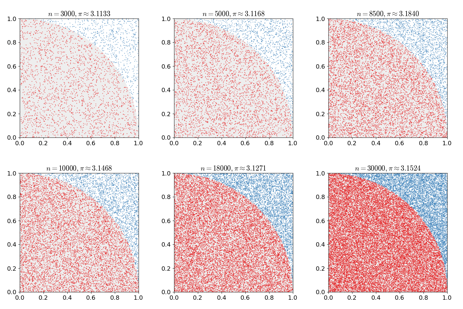
A Monte Carlo simulation is one in which we have a problem that we know how to simulate but not how to solve for directly. Heres an example: We want to compute a value for \(\pi\). Well, it's not exactly straightforward to do that. However, it's extremely easy to randomly place points on a cartesian coordinate grid, calculate if \(x_i^2 + y_i^2 < r^2\), and estimate based on ratios the area of a circle with radius \(r\). If we place enough points, we can just solve \(A=\pi r^2\) for \(\pi\)!
By being smart about the problem we simulate, and being a bit clever in how we interpret the observed outcomes, we can infer solutions to the problem in question.

Monte Carlo simulation to estimate the value of pi.
Now we just need a clever way to apply that to games. Let's say we're playing tic-tac-toe. To apply Monte Carlo search it, I'll just make a tree of all possible move combinations starting from an empty board, play out dozens of random games, and we'll observe that certain branches have more cumulative wins than others. These we say are the better moves. And thus, without any sophsticated methods, we have devised a game plan from simply observing simluated actions. This method is called Monte Carlo Tree Search, or MCTS.
The Chess Problem
Unfortunately for us, there are more Chess positions than there are atoms in the universe. This makes building a tree of random games either impossible or incomplete and not particularly useful. Our solution to this is to be highly particular as to which positions we explore. If we can find a way to estimate how good a position is then we can cue our search down only good lines and avoid wasting compute on less useful ones.
The Neural Network
The way we pull this off is with a large neural network that we train to approximate how good the lines are for a given board position (\(S\)) that we feed it. This network then outputs 2 values: a policy (\(\pi\)) and a value (\(v\)).
The Policy \(\pi\): [Vector] <\(p_1,p_2,p_3,...,p_n\)>
A policy vector is generated for each position that aims to give us the likelihood that we should take move \(a\) for each move possible in \(S\). Our motivation is to train the network such that good moves get higher probabilities. This provides quality information about where to start searching even before exploring any of the possible lines. Enough training of the network and these values become highly accurate, predicting the top engine move around 50% of the time with no search performed.
The Value \(v\): [Float] \(v_S\)
The network will also yield a value \(v\) for each \(S\) - unless \(S\) is an endstate in which case we use the actual outcome. \(v\) is clipped from -1 to 1, being interpreted in the same way as a traditional engine evaluation would be. A higher value means better odds for white, and a negative value means better odds for black. The value gives us a way to assign scores as we search down a branch of moves. Because outcomes are so sparse in chess, we need a heuristic that applies to non-endstates so we can add up the values as we explore down a tree.
The PUCT Algorithm
The final piece in performing MCTS is deciding which lines to search in a given position. Now that we have some predictors to help guide us, we'll fit them together using a scoring system called PUCT (Polynomial Upper Confidence Tree). Search on a position is performed a given number of times (800 used in the paper). Each iter, we calculate a score for each \(a\) that encourages searching moves that are either promising or currently under-explored. The move with the highest score is selected for search, all PUCT values are recomputed based on the results, and we repeat n_iter times. Here's the formula used, lets break it down.
\(PUCT(S,a) = Q(S,a) + c_{\text{puct}} \cdot P(S,a) \cdot \frac{\sqrt{N(S)}}{1 + N(S,a)}\)
- \(Q(S,a)\) - the sum of all \(v\)'s discovered after taking move \(a\)
- \(c_\text{puct}\) - a constant used to adjust exploration vs exploitation
- \(P(S,a)\) - the probability assigned to this move by the model
- \(N(S)\) - number of iterations run so far (down any move)
- \(N(S,a)\) - number of iterations down \(a\) epecifically
As you can see, more promising moves (based on higher \(Q(S,a)\) or \(P(S,a)\)) will get higher scores - and well search them more. Additionally, neglecting a line will push up its \(\frac{\sqrt{N(S)}}{1 + N(S,a)}\) value, and we'll be sure to not leave any move completely unexplored.
Making a Move
After running our search iterations, we interpret the moves based on visit counts. The more a move was visited the more its probability value and its observed outcomes outweighed those of other moves. If we're in an exploratory mood (i.e. during training), then we normalize the move counts and sample the next move using the resulting vector as weights. If we want just the best move then we just pick the most visited move.
Training
To effectively train the network from scratch, the model plays games against itself and accumulates a dataset of (\(S\),\(\pi\),\(z\)), where \(z\) is the observed outcome of the game. Once we've generated thousands of games, we train the model to produce a policy that mimicks the observed \(pi\) and values that mimick \(z\).
Two things of note here: during search, both \(pi\) and \(v\) are useless. All signal comes from explorations that had actual endgames in their trees. This is the only thing that would cause meaningful nudges towards preferring those lines. Training is thus initially very slow, and hundreds of thousands of positions are required to bootstrap the model.
Second, noise is introduced by training the model to predict the final game outcome for all positions in that game. I.e. even the opening move is trained on the outcome which may be completely unrelated. This is mitigated, though, because if that position indeed had nothing to do with the endgame it would be trained an equal number of White and Black wins - thus the noise gets cancelled out.
Continue on to Part 2
Next iteration, we'll build the algorithm in Python!
